Project report
The workflow of the project
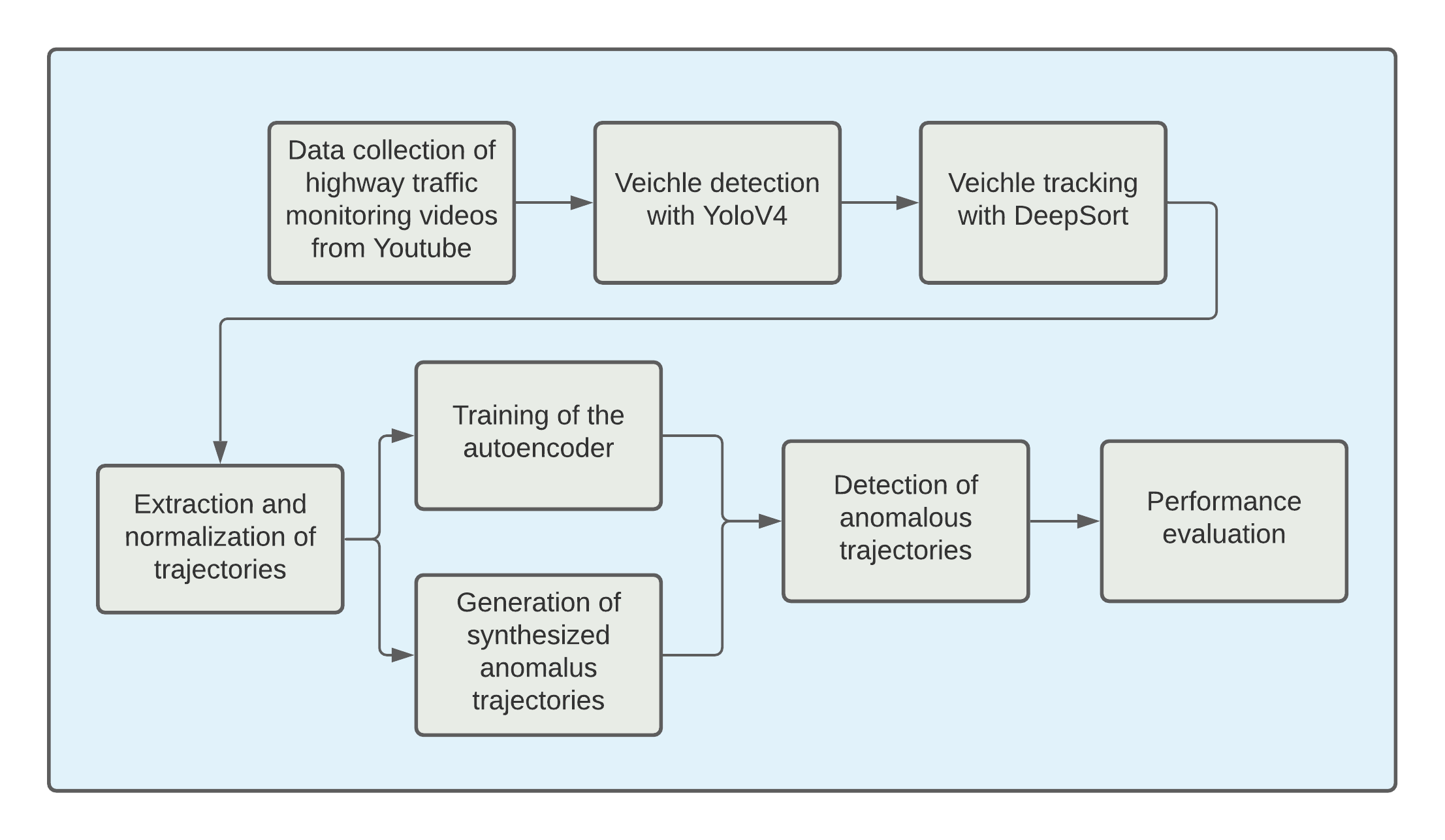
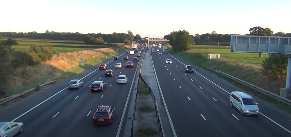
Data collection
Our first problem concerns data collection. We could not find annotated data for our task, so we collected videos from YouTube of highway traffic monitoring.
In the collected videos, there are a lot of vehicles such as cars, trucks, and motorcycles that are moving at the same time and need to be tracked in order to obtain trajectories and later recognize anomalies in driving behavior.
For this reason, an algorithm for multiple object tracking (MOT) must be used, but first the vehicles must be detected.
Veichle detection and tracking
When it comes to object detection, there are many algorithms such as Mask R CNN
(He, Gkioxari, Dollár & Girshick, 2017), Faster R CNN (Girshick, 2015), SSD (Liu et al. 2016),
YOLO (Redmon, Divvala, Girshick, & Farhadi, 2016), etc.
An object detector that can detect in real time multiple objects in a single frame, that is multiple vehicles, is YOLO.
In this case, we used the new YOLOv4 to detect the vehicles, and then, we used the obtained detection to steer the tracking process using the Deep SORT tracking-by-detection algorithm.
The goal of the tracker itself is to associate the obtained bounding boxes in different frames together so that the boxes containing the same vehicle are assigned the same unique ID.
To this end, the tracker may use the information it can obtain from the detected bounding boxes, e.g. the locations of box centroid, their dimensions, the relative position from the boxes in previous frames, or some visual features extracted from the image. In addition, it uses the information about appearance of the tracked objects and considers only information about the current and previous frames to make predictions about the current frame without the need to process the entire video at once which makes DeepSORT an online tracking algorithm
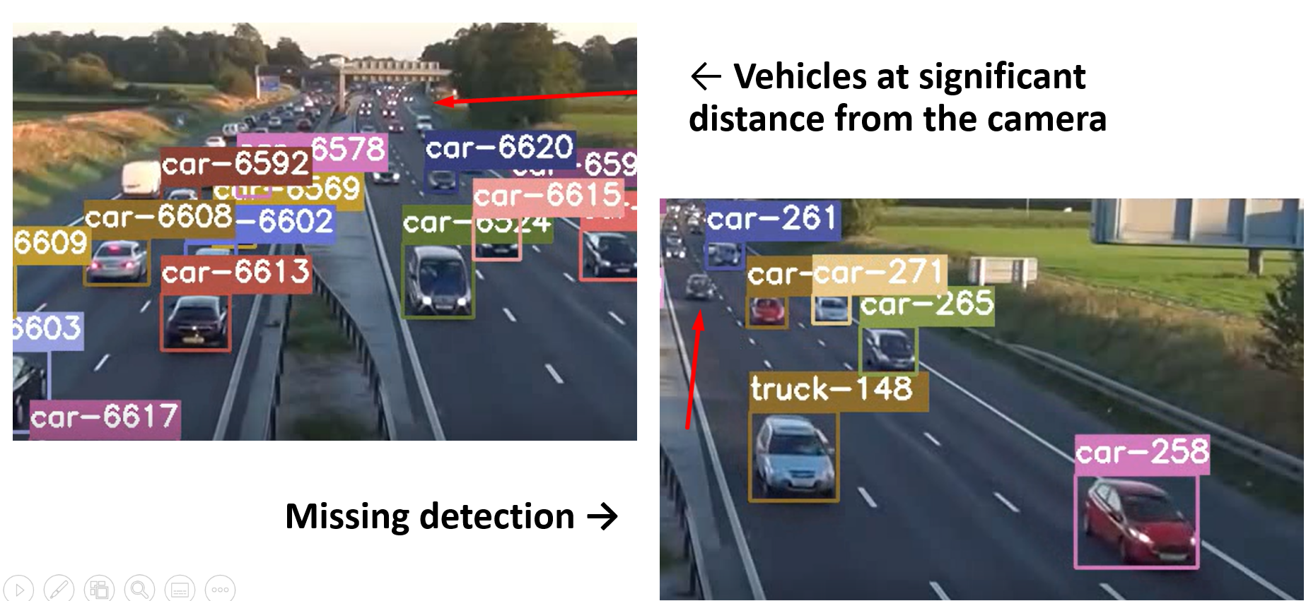
The problems with detection and tracking
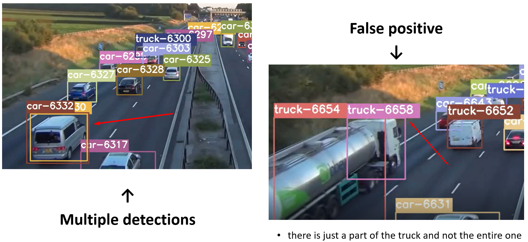
Tracking is greatly influenced by the accuracy of the object detector. If a vehicle is inaccurately detected, the tracking will be inaccurate as well. For example, false positives of the detector, i.e. the bounding boxes that are detected where there are no vehicles to detect, can confuse the tracker to assign an ID to that box that would otherwise have been assigned to a correct detection. In other cases, the false positive will produce spurious object IDs with short track durations.
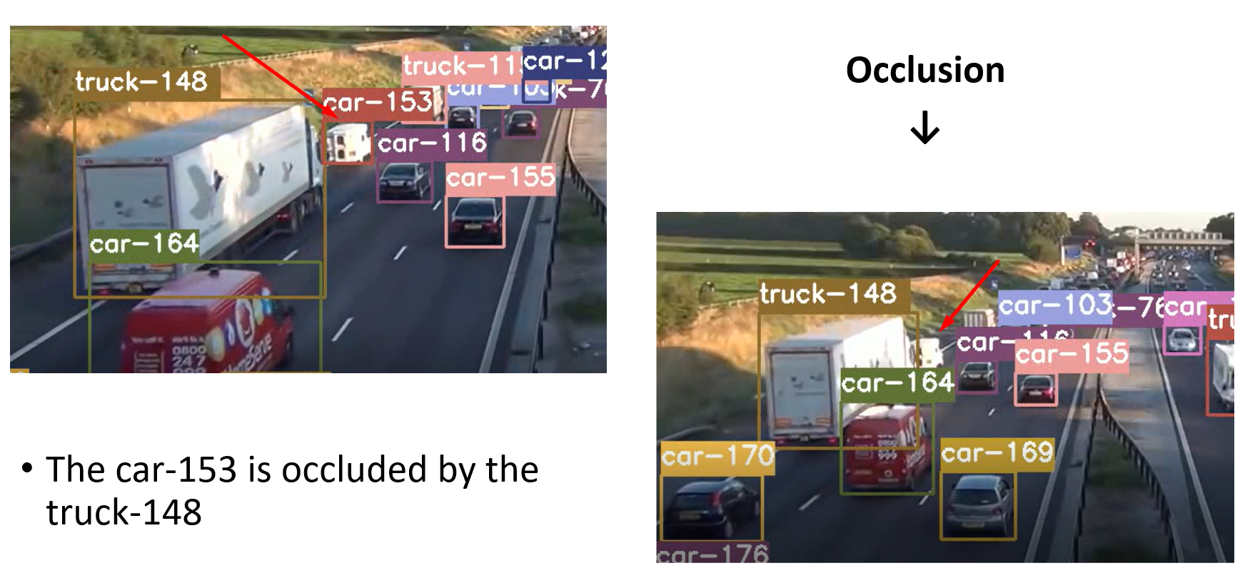
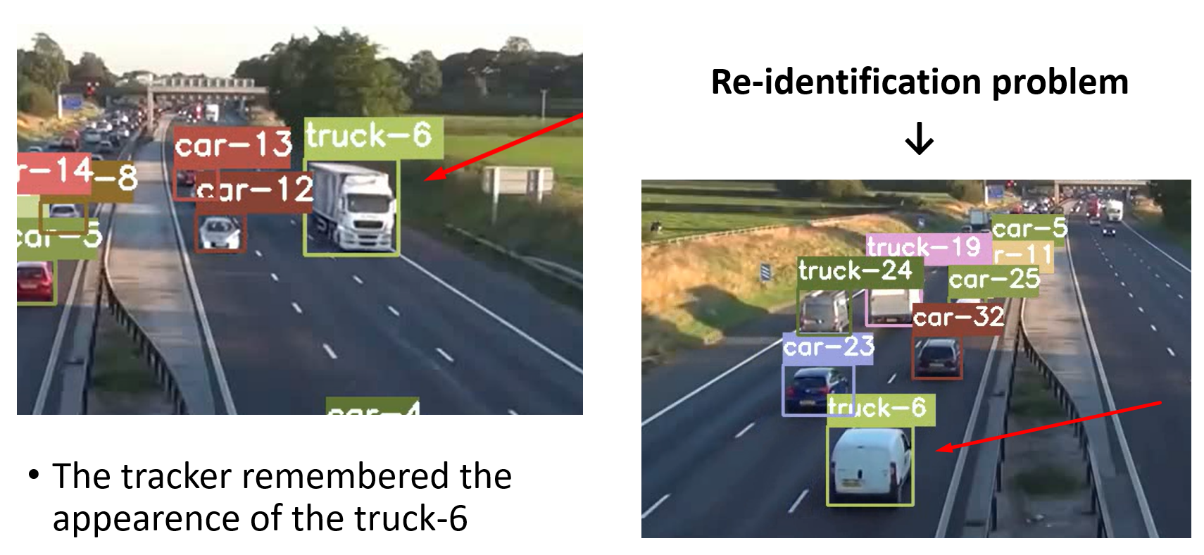
Also, the detector may fail to detect vehicles when they are at a significant distance, and in such cases they cannot be tracked for the entire region they are supposed to traverse. Additionally, there are identity switches due to occlusion or similar color and shape of the vehicles, together with the possibility of re-identification of a vehicle that is actually a new one.
Also, in various weather conditions, such as rain, there is poor visibility, making it difficult to detect and track all the vehicles as on a sunny day.
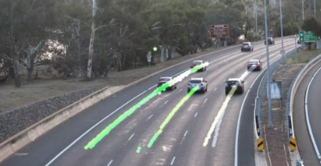
Extraction and normalization of trajectories
From the output of DeepSORT, we then extracted the trajectories of each vehicle, but to avoid the previously mentioned problems,
we imposed some constraints.
If for a fixed number of frames, the track ID does not appear (exceptionally large detection gaps), and then after it reappears again, we are presuming the same ID was used on multiple vehicles and then we split the trajectories into separate trajectories. After that, for each obtained trajectory we verify it in a way that we discard it if it is smaller than a desired length or if it contains a gap without detections larger than 20 frames. Also, if there are fewer missing frames, we added values in between.
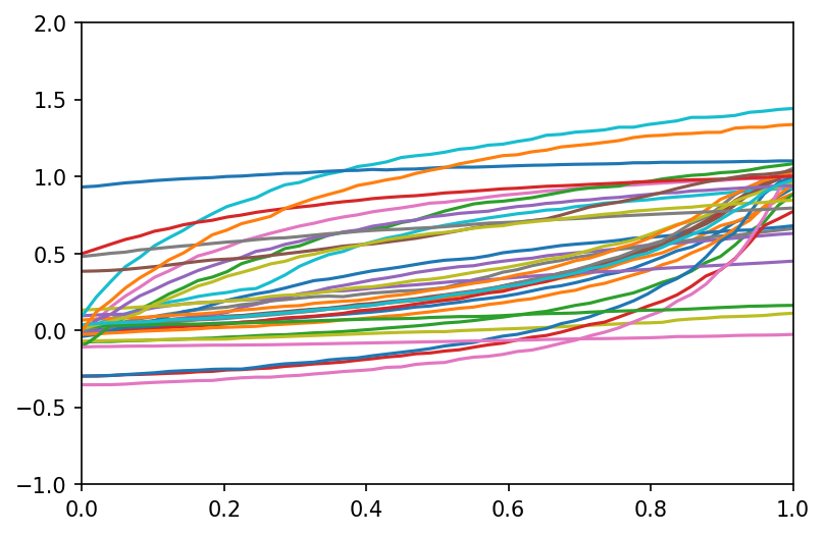
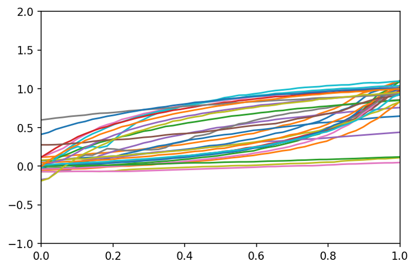
The trajectories are arrays with x,y, t coordinates. We regularized them all to have the same number of timepoints, equally spaced out (numpy interpolation)
As the result we have multiple lanes going in different directions
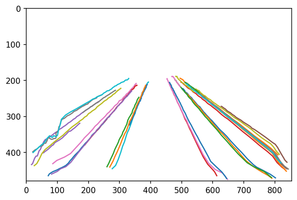
Then we plotted the starting and ending points of the trajectories, and run a clustering algorithm (OPTICS) to find typical entry/exit regions
We used OPTICS because it does not require the number of clusters prespecified and it
discards some points as outliers.
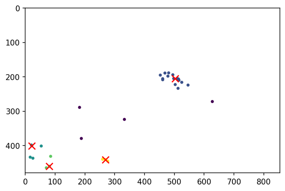
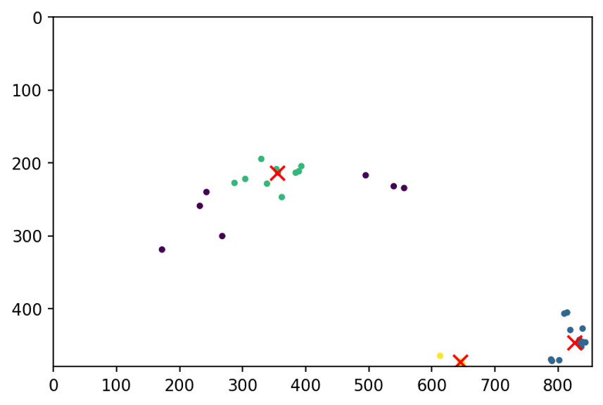
Then we connected the corresponding entry and exit points to get the common connections (The count how many trajectories use each entry-exit pair)
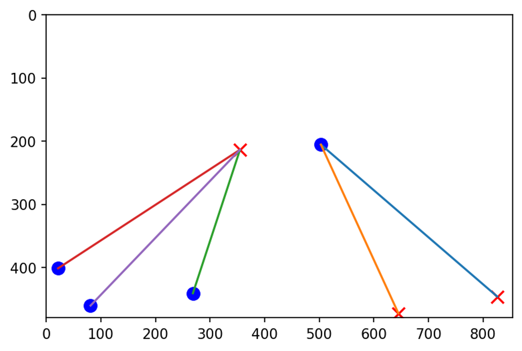
We renormalized the coordinate arrays of each trajectory based on how similar they are to the closest matching connection
(Minimal distance between starting/ending points of the trajectory and the cluster median), we rescaled the coordinates so that the median entry point of the connection is (0, 0) and median exit point is (1, 1).
**On the left (x-t), on the right (y-t)
Synthesizing anomalies
The renormalized trajectories can be used to more easily generate anomalous trajectories based on real ‘normal’ ones. The examples we perform are:
the vehicles stop for a random amount of time in the middle of the road,the vehicles suddenly speed-up for a brief period of time,
the vehicles are driving in reverse, the vehicles moving toward another median exit point (unstandard connection),and the vehicles starting from a different entry point.
Variational Autoencoders
Variational auto-encoders (VAEs) are particular auto-encoders designed to have continuous latent space, and they are therefore used as generative models. Instead of directly extracting the code corresponding to an image, x, the encoder of a VAE is tasked to provide a
simplified estimation of the distribution in the latent space that the image belongs to.
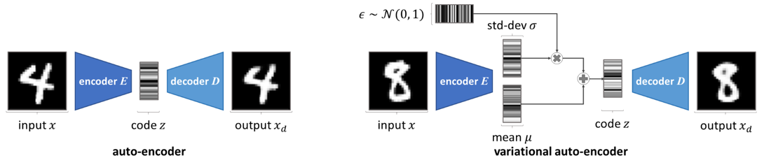
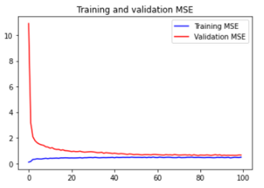
During training, a loss—usually the mean-squared error (MSE)—measures how similar the output image is to the input one, as we do for standard auto-encoders. However, another loss is added to VAE models, to make sure the distribution estimated by their encoder is well-defined. Without this constraint, the VAEs could otherwise end up behaving like normal auto-encoders, returning variance of null and mean as the images’code
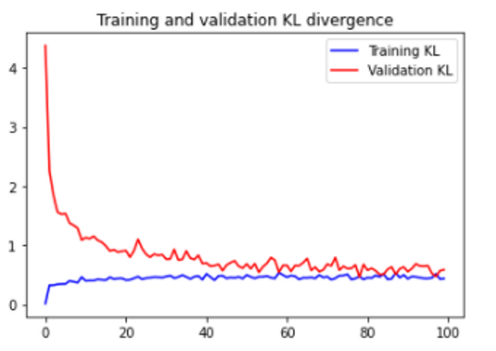
This second loss is based on the Kullback–Leibler divergence (named after its creators and usually contracted to KL divergence). The KL divergence measures the difference between two probability distributions. It is adapted into a loss, to ensure that the distributions defined by the encoder are close enough to the standard normal distribution.
Our autoencoder receives one dimensional Input x,y coordinates for time t. The architecture uses Convolutional Layers and one Dense layer to represent the latent vectors for estimating the distribution of the input data.
We use kernels with width of 6 in order to capture the dependencies between near points in time. The kernel’s high in the first layer is 2 and the stride is 2 in order to capture the x and y relation.
Our network has around 17 thousand trainable parameters.
The results
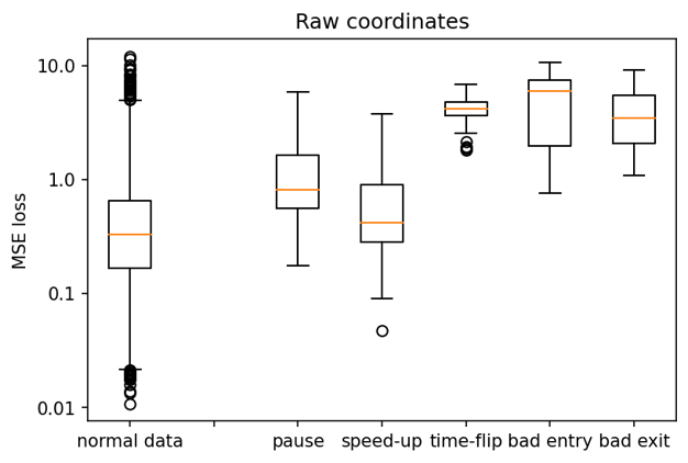
We have trained the variational encoder on an approximately 30 min long sequence of normal highway behaviour. Two variants were trained, one on ‘raw’ x-y trajectories (here a simple 0-to-1 normalisation was applied on the values range) and another on the ‘normalized’ set of trajectories (prepared as described above).
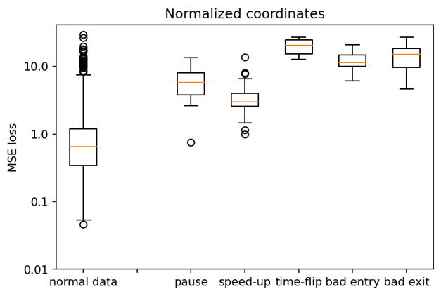
We evaluate the performance of the two variants by comparing how distinctly they score normal and anomalous trajectories (the score is the MSE loss between the original and the vAEC reproduction). The normal set is the set of trajectories used in the training. The anomalous sets are artificially synthesized as described before.
We find that the distributions of scores on normal and anomalous trajectories do differ, although there is a significant overlap in their distributions. The autoencoder working with ‘normalized’ trajectories shows somewhat better results, withe clearer distinction between normal trajectories and the anomalous trajectories involving cars stopping or speeding-up.
We also do a ‘real-world’ test by scoring the 3-min cut-out from the same video in which a traffic jam occurs (this part was not used in training). This sample cannot be compared in the same way as the artificially prepared ones, as it also contains many normally-behaving trajectories. We rather do a more fine-grained comparison of the loss-score histograms.
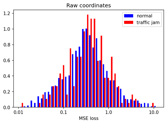
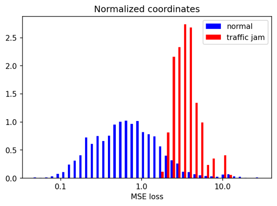
Here the results are less clear. The ‘raw’ autoencoder version does not produce visibly distinguish between the training set and the traffic-jam containing sequence. The ‘normalized’ autoencoder produces two clearly different distributions, with the traffic jam distribution containing two modes (presumably from normal trajectories and traffic-jam ones) - both of which differ from the training set distribution.
********** You can find our code
here **********